

The Nyquist diagram with Ti-84 Plus (CE)
Explanation of the use of the Nyquist plot with a Ti-Basic program
Using this program needs knowledge of the Nyquist theory
Nyquist's diagrams are very important in control system theory. With this Ti program, you can plot Nyquist diagrams and analyze for example the phase and gain margin of a motion control system.
A control system usually consists of a process: Hprocess and a controller: Hcontr which ensures that the output Uo follows the input Ui as accurately as possible. However, systems can be unstable for certain frequencies. To guarantee a stable system, the phase margin and gain margin are defined in control theory based on the fact that Hcontr*Hprocess for each frequency has a certain phase and distance to the point -1. If Hprocess*Hcontr = -1, then the denominator of Uo/Ui is equal to 0, resulting in Uo/Ui being equal to ∞ (unstable). Hprocess*Hcontr is referred to as the open loop transfer function.
Schematic representation of the system

The Nyquist diagram of an open loop transfer function represents the open loop gain and phase as function of frequency and gives insight into the stability of control systems.
As an example, we have the open loop transfer of a motion system with the function :
H(s)=Hcontr*Hprocess = Hcontr*2.071/{(0.0188s)(s+.01s)(1+0.001s)}
A first run is done to gain insight into the stability of the process for Hcontr =1
For more details of the system, visit the pages Bode diagram 1 and 2.
Phase margin and gain margin are widely used to observe how stable the system is.
With the Ti- program, phase margin and gain margin can be calculated and the value of Hcontr can be adjusted afterwards to meet the desired phase and gain margin.
In the Ti-program we have to substitute for s=iT where i = imaginary vector of length 1.
T stands for omega =2*π*f. So T is the radian frequency (rad/sec).
The Bode diagram for the same transfer function as for Nyquist is shown on the page Bode diagram and gives the same results and conclusions. After using the programs NYQUISTE run the program Adefault to reset your Ti.
For the input H(s=iT) take care to use the correct brackets. Scaling has to be chosen, and then a plot will appear. You can adjust the scale afterward to plot your diagram in the area of interest.


For a length of R=1 and Hcontr=1, the phase is -134.83°. This is exactly the same value as calculated with the Bode diagram and results in a phase margin of 180° - 134.83° = 55.17°.
To obtain a phase margin of 60°, the phase should be 120° (119.94° in the figure) at a frequency of 51 rad/s.
The total gain should then be 1, but equals 1.92 if Hcontr=1, so the proportional gain Kp of Hcontr has to be adapted according to 1/1.92=0.52 (the same as in the Bode diagram). Adding the PI controller by Hr(s) = Kp+ 1/(taui*s) with Kp=0.52 and taui=0.38 sec gives next Nyquist diagrams. On the page Bode diagrams page 2 an explanation is given how taui (=0.38 sec.) is calculated

As already explained on the Bode diagram page, the PI-controller gives five degrees less phase margin (180° - 125.61° = 54.39°) but eliminates static disturbances. The results of the TI-84 are in accordance with those of Matlab.
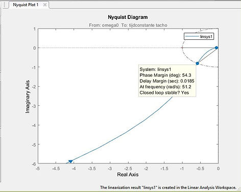
Results obtained with Matlab
Download the program NYQUIST2.8XP:
Further explanation of the Nyquist stability criteria using the Ti-84
More background information on the Nyquist criteria and the application of the Ti program Nyquist2 .8XP
During the time, the original program has been improved, and more explanation will be given.
The Nyquist stability criteria is defined as a graphical technique used in control engineering for determining the stability of a dynamical system.
In short, a system is stable if the point -1 in the complex plane is to the right of the open loop transfer function if ω varies from -∞ to ∞ rad/sec. The Nyquist criterion will be made clear by means of an example.

The open loop transfer function = Hcont*Hprocesss. This function is plotted in the complex plane
for s= jω varying ω from -∞ to ∞ rad/sec
Suppose Hcont*Hprocesss=120/{(s-2)(s+6)(s+8)}.
This function must be entered in the program as follows, see Fig.1. For the first run, it is not always easy to choose a satisfying under and upper limit for ω and the step value. But after a run, see Fig 2 if the plot does not satisfy we can correct that, see fig 3 and 4 and choose lower limits and a smaller step for ω. A much better plot arises. Although fig 2 is not very accurate, we can already conclude that the system is stable because the point -1 is situated at the left of the curve for ω -∞ to ∞ rad/sec. At the end, we choose another amplification factor. Instead of 120 we choose 90 which results in an unstable system.
The point -1 now situated at the right of the curve for ω -∞ to ∞ rad/sec and therefore the system is unstable. It cost some processor time before the Ti starts plotting.
